Oddities and Queries in MS Excel – Review001

 

We know that problems frequently arise with spreadsheets. Usually these problems are referred to as errors and give spreadsheets a bad reputation. The aim of this series of reviews is to examine these potential problems in greater detail, using the ACBA Mapping software as the starting point for the investigation.

This first review looks at a single file from the collection of excel files deriving from the collapse of the Enron Corporation. This particular file gave rise to a wide variety of interesting conundrums and offers a starting point for this series of reviews. The issues arising from this file are considered under the following headings.

• Interrupted column formulae
• Displaced formula
• Extended use of formulae 
• Irrational references
• Unusual column data sequence

The “BR New York ticker 10_01” spreadsheet comprises 18 worksheets, 17 of which are visible and have been mapped. Several of the worksheets have almost identical structure. The review below uses examples from a single worksheet where identical issues may be repeated over several sheets. A zip file of both the original workbook and its associated map file can be downloaded from here.

Many of the issues described are portrayed via a “map” of the spreadsheet. The ACBAMapping software is an Excel Add-In which is available for download without charge.

Interrupted Column Formulae

Interrupts Case 1

As a general rule, where repeated column formula is interrupted by a new formula, it is noted by a green triangular marker in the top left of the cell. Unfortunately, a spreadsheet, such as 'ZONE A OFFPEAK', can be littered with a number of these green markers as in this case. Not all these markers are particularly meaningful. However, the figure below circles the particular cell that causes us concern in red.

Figure 1- Several cells in ‘ZONE A OFFPEAK’ have green markers.

The section of the cell map below highlights the locations of two generic formulae – F11 (=MyRef) coloured sky blue (Azure) and F3 (='EOL LINKS'!MyRef) coloured navy blue. The F11 block is interrupted by F3 which calls for data from another sheet ('EOL LINKS').

Figure 2- Highlights where a specific block of formulae is interrupted

While this does not necessarily indicate an error, it certainly calls for further investigation. Using the Microsoft’s auditing function (Trace Precedents), we can see that while the majority of formulae pick up the preceding value in the column some of the cells source their data from 'EOL LINKS'. Curiously, the data from ‘EOL LINKS’ is not called sequentially.

Figure 3 - Separate sheet links are not sequential

The five calls have the cell sequence I6, I6, I7, I5, and I4. There is no obvious logic for these calls and, from an auditor perspective, would deserve querying with the spreadsheet builder.

Interrupts Case 2

This comes from the same worksheet - 'ZONE A OFFPEAK'. I noted that the penultimate column in this range had some unusual formulae – e.g. F20 (=(MyRef+MyRef+MyRef)/3). The detail of the range appeared as shown in Figure 4. (The source cells are not visible within the figure.)

Figure 4 - Example calculation in Column CY

This was sufficiently odd to examine the whole table in more detail. An extract from the cell map is shown in Figure 5.

Figure 5 - The cell map associated with the table in Figure 4

The first thing that hits the viewer is that the presentation is unusually irregular. This level of irregularity is not evident on inspecting the original spreadsheet. Not surprisingly, this irregularity is also evident in the list of generic formulae.

Figure 6 - Formula list associated with column CY highlighted with red outlines

We can see a similarity in the structure in all, bar one (F10), of the highlighted formulae. Looking at the formulae F19 and F20, they are given the general structures of [Gen: =(MyRef)] and [Gen: =(MyRef+MyRef+MyRef)/3]. F19 could be re-written =(MyRef)/1 without changing the logic of the formula. There appears to be a standard structure to this formula where the number of collection points (MyRef) is the divisor for the formula. Testing this standard structure for all the other highlighted formulae (except F10), shows this to be true.

Nevertheless, we can see from Figure 5, that the shape of the collection points is very irregular. I needed to test whether a formulae with the divisor ‘n’ always had the same shape.

I tested formula F4 [Gen: =(MyRef+MyRef)/2] from Figure 6. It is represented in the last but one column of Figure 5 and is shaded in grey. There are five cells with this general formula. Four of these take their data from user input (U) circled in red in the middle of the table. The fifth takes its data from the predefined constants (C) in the first 5 columns. Clearly, the generic shape of the formula does not determine the equivalence of the source of data.

Formula F10 has the shape [Gen: =IF(AND(MyRef=0,MyRef=0),0,(MyRef+MyRef)/MyRef)] and is quite different to all the formulae in the rest of the column. We need to look at the formula in its original context. Figure 7 below identifies the sources of data for one of the formulae F10.

Figure 7 - Sources of data for the formula F10

This formula was clearly never used. We need to surmise why it was considered appropriate initially. My best guess is that the spreadsheet builder recognised that the formula he had devised wouldn’t work in all cases, so he used the work arounds we discussed above.

Bearing mind that this workbook was created around 2001, long before modern formulae such a SPLIT were available, this solution, although inelegant and potentially error prone, did the job.

Interrupts Case 3

This case comes from a fairly innocent looking table in the worksheet ‘Zone J Offpeak’. This pictured below.

Figure 8  - An apparently straight forward table from 'Zone J Off peak'

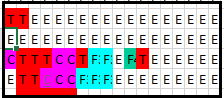
The primary formula for this block has the form Gen: ='Zone J'!MyRef (F12), which clearly takes data from a separate worksheet. However, the highlighted block of the range covered by this formula (Figure 9) shows that the first column is interrupted by hand posted constants. They are all zero.

Figure 9 - Map of 'Zone J Offpeak' - formulae (azure) interrupted by constants (magenta)

While there may be a perfectly reasonable explanation for the hand written addition of zeros. That explanation should surely be made explicit.

Interrupts Case 4

The extract of a cell map comes from the ‘Spreads’ worksheet. The first two columns of each data block all use the general formula F1 (Gen: =DATA!MyRef), but the very first cell on this map uses the general formula Gen: =+DATA!MyRef.

Figure 10 - Why the change in formula presentation?

This has no impact on the calculation of the worksheet. But why did it happen in the first place?

Displaced formula

Mostly, formulae of the same generic type get used in the same area(s) of the worksheet. Occasionally a formula of a particular type gets used in a clear region and gets used again in an isolated cell.

Displaced Case 1

In this case the map (Figure 11) shows a column of a single generic formula towards the left. There is also a single instance of it on the right.

Figure 11 - Why is there an isolated formula towards the right?

While this is not an obvious error, it certainly deserves investigation. It turns out that this formula is identical to those considered in the discussion at Interrupts Case 1 and in the same location. Given its position in the penultimate column, it is almost certainly valid.

Displaced Case 2

In this case, the displaced formula occurs at the bottom of a column.

Figure 12 - A single, formula at the bottom of a column of text values

The original spreadsheet does not give much clue as to why a column of 0’s, should end in in a formula – see Figure 13.

Figure 13 - Why should a column of text 0’s end with a formula?

Some queries are inevitably left unanswered, as in this case where we have no access the workbook ‘NYPosMgr.xls’.

Extended use of formulae

Some formulae appear to be used again and again in a variety of different locations and having a variety of shapes as highlighted on the map. The most common instance of this is the formulae =MyRef.

Extended Case 1

This case derives from the map sheet to the worksheet ‘Sum Positions’. On this map formula F3 has the general structure =+MyRef. It has a variety of roles, but in this case it is repeating a series of five column headings. The purple constants on the same row represent the source of those headings. However, its most general use is carry over numeric values.

Figure 14 - Extending the use of Text Headings

Formula F4 on the same worksheet has the same role, but is given the structure =MyRef. One might speculate without success as to why this small difference was introduced.

Extended Case 2

The source of this query is the map to the worksheet ‘ZONE A OFFPEAK’. Formula F2 (Gen: =MyRef-MyRef) extends a couple of rows beyond it expected finish point. The finish point might be expected as the lowest row of the formulae mapped in azure F1 (Gen: ='ZONE J DAY AHEAD'!MyRef).

Figure 15 - The right hand highlighted column extends beyond its expected position.

This is an oddity arising out the way the spreadsheet was built. It does not suggest an error at this juncture, but it could introduce errors if the structure of the spreadsheet was reused.

Irrational References

Spreadsheets are used almost universally as tools in public and commercial businesses. Of their many advantages, speed of construction and presentation is certainly close to the top of the list. This need for speed frequently leads to the use of shortcuts. On review, some of these shortcuts look distinctly odd and potentially wrong.

In the case of worksheet ‘ZONE A DAY AHEAD’ there was nothing out of the ordinary until I looked at the map.

Figure 16 - The constants (coloured purple) from worksheet ‘ZONE A DAY AHEAD’

The cell map identifies all cells that are employed as sources for formulae elsewhere within the sheet. Cells that are empty are regarded as ‘User entry’ cells coloured yellow. While those that contain any value are treated as ‘Constants’ and are coloured purple.

In this instance, the cells marked as ‘Constants’ had an unusual shape. Row 19 of Figure 16 looked sensible, possibly numeric values underneath a heading. But why was there a single constant in row 21.? Assuming row 22 is also a heading, why weren’t all the values underneath included as a constant in a formula. This deserved further investigation.

Figure 17 - The original 'ZONE A DAY AHEAD'

The original spreadsheet looks much more regular than its associated map.

Irrational Case 1

In this case concerns two similar formulae, F1 (Gen: =AVERAGE(MyRef:MyRef,MyRef:MyRef)) and F2 (Gen: =AVERAGE(MyRef:MyRef,MyRef). Both formulae draw data from two locations, one of which is empty.

Figure 18 - Formula F1 draws data from two

Figure 19 - Formula F2 draws data from two different sources

 

For both formulae, the data sources are not even the same size. While this is not proof of an error, it is certainly cause for further investigation.

Irrational Case 2

Formula F4 is a simple average Ex: =AVERAGE(A9:L15), but, as we can see from Figure 20 (below), it includes empty cells (in yellow) and constants (magenta).

Figure 20 - The map of the source data for Formula F4

This appears to suggest that on the 4^th row of constants there were 2 “text” values that were not included. I wondered whether this was deliberate.

Figure 21 - The source spreadsheet for Figure 20

This shows that many of the so-called constants were text headings, but the majority of the cells in the range are empty (marked in yellow on the map above).

The map raises questions that cannot be answered from two decades later.

• Why limit the average to the columns headed HE1 – HE12?
• Was the author really expecting values in the empty cells?
• And, if so, why?

It also highlights one of the characteristics of many Excel formulae. When manipulating numeric values (e.g. AVERAGE) the formula will simply ignore blank cells or text values. This allows for spreadsheets to be built very quickly, but does not always maintain their logic.

Unusual Data/Formula Sequence

The common way of build spreadsheets is to have one formula per column, with, perhaps, a total at the bottom. Other approaches include the use of sub-totals. When, I first encountered these particular examples, I expected an issue similar to that described in ‘Interrupts Case 2’.

Sequence Case 1

The map to the worksheet named ‘Marks’ looked rather uninteresting, until I noticed at strange set of repetitions in the formulae for the right hand block of analysis.

Figure 22 - Repeated sequences of formulae in the right hand block

You will see that the sequence of formulae in the right hand block (enclosed in yellow) is repeated two more times in this image and is started a 3^rd time. This was so odd that I reviewed the source worksheet.

Figure 23 - The 'Marks' spreadsheet showing the pattern of calculation

The sequence of calculation is determined by the sources being collected. The pattern is certainly strange, but it is not necessarily wrong.

The repetition of the sequence arises from the years being reviewed. The final year 2005 is missing some data hence the pattern stops there.

Sequence Case 2

In this case there is no obvious logic to the sequence of references within a single formula. This prevents the user from using the Excel’s copy and paste facility. I noticed this as a result of investigating the unusual lay out of constants within the worksheet (“EOL LINKS”).

Figure 24 - The constants do not marry up with the Formulae

The constant (background colour purple) do not match the formulae cells (in green). In order to determine why I had to review the original worksheet. This showed that adjacent formulae did not have a regular sequence of references.

Figure 25 - Adjacent formulae do not have a regular sequence of references

The formulae in the worksheet “EOL LINKS” must have been posted by hand, which makes them much more prone to error. In fact, there are no obvious errors revealed in this worksheet.

Summary

In this single workbook, we have identified a range of oddities. A few of them, if not spotted in time, could lead to errors. The remainder are interesting because they highlight the practical approaches we take to constructing both an individual spreadsheet and a whole workbook. However, it seems clear from this review that the workbook never came into active service before the failure of the Enron Corporation.

I had assumed that the Enron collection would contain all the relevant files needed for the analysis of any individual workbook. However, the Displaced Formula, Case 2 identifies that this is not true. There is no file called ‘NYPosMgr.xls’ in the collection. Care must be taken, when calling values from other files, to ensure that the most up to date value is always available.